j-intro

J

What?

J is a programming language with roots in APL. You can find it here.

Getting the ball rolling

Once you have installed the package, start up J Term, which is your interactive interpreter.

To get the most of this, I suggest going straight for the labs. Those aren’t installed by default (they live under Help -> Studio -> Labs). To do so, go to Tools -> Package Manager.

j_install_labs

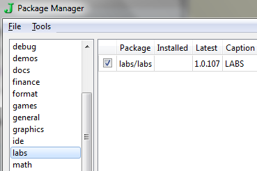
Select category at the bottom and click on labs. Press Install.

Updating server catalog...
Done.
Installing 2 packages of total size 694 KB
Downloading base library...
Installing base library...
Downloading labs/labs...
Installing labs/labs...
Done.

(I used this opportunity to update my base system).

Go back to the labs module and select ‘A J Introduction’:

To run this lab, first install: graphics/plot, graphics/viewmat

Bummer - it needs some more package. Let’s not take any chances. Run the J Console (that’s different from J Term) and type: install'all'. Now if you were thinking you could just do something like install'graphics/plot', I’ll stop you right there and save you a couple of minutes - you can’t. The install cmd only takes two possible arguments - 'all' or 'qtide' . To close the console, type exit''.

Okay so that might have been a little rough - but it does get better. I suggest going through that lab first before reading on, otherwise it might not make much sense.

J <-> Python

Just like when learning a foreign language you have a tendrency of using your native one as reference, it can help to map J to something you’re familiar with to get started.

Python	J
`x=2`	`x=:2`
`2*2`	`*:2`
`map(lambda x: x+2, [1,2,3])`	`2 + 1 2 3`
`range(10)`	`i.10`
`[x*2 for x in range(4)]`	`(i.4) ^ 2`
`6/4`	`6%4`
`lambda x: 1/x`	`%x`
`math.exp(3)`	`^3`
`math.log(10)`	`^.10`
`math.log(math.exp(1))`	`^.^1`
`sum(range(5))`	`+/i.5`
`[a+b for (a,b) in zip([1,3,5],[2,4,6])]`	`1 3 5 + 2 4 6`
`[0,1,2,3][-1]`	_1{i.4`
`math.sqrt(2)`	`%:2`
`lambda x: x+x`	`+:`
`[1,2,3].append(4)`	`1 2 3, 4`
`len([1,2])`	`# 1 2`

Cool examples

  12 10 +. 8 8 NB. GCD
3 2
  4 3 2 1 >. 1 2 3 4 NB. greater-of
4 3 3 4
  +/1 2 3 4 NB. insert + between each element and evaluate
10
  (i.2) +/ (i.4) NB. this creates a 2x4 table
0 1 2 3
1 2 3 4
  H=:%(1+x+/x) NB. Hilbert matrix, where x=:i.4
  H
1         0.5       0.333333  0.25      0.2
0.5       0.333333  0.25      0.2       0.166667
0.333333  0.25      0.2       0.166667  0.142857
0.25      0.2       0.166667  0.142857  0.125
0.2       0.166667  0.142857  0.125     0.111111

Okay now for some cooler stuff!

  <1 NB. that's the 'box' operator
┌─┐
│1│
└─┘
  <\i.4 NB. this will box successive iterations
┌─┬───┬─────┬───────┐
│0│0 1│0 1 2│0 1 2 3│
└─┴───┴─────┴───────┘
  x=:1+i.5 NB. that's 1 2 3 4 5 
  +\x
1 0 0 0 0
1 2 0 0 0
1 2 3 0 0
1 2 3 4 0
1 2 3 4 5
  +/\x NB. we can see this as summing each row
 1 3 6 10 15
  avg=: +/ % # NB. read the next line for this to make sense!
  avg 1 2 3 NB. this gets executed as (+/ 1 2 3) % (# 1 2 3) - so sum / number of elements
2

Before I forget…

no verb precedence and right-to-left evaluation

[insert example with mult]

scope - =: vs =. (global vs local - can define global inside a fn), primarily used for debugging it seems

When defining in a script, use =: otherwise =. would make them local to the load verb

Locale & Scope

I think J uses the name locale for what some people might consider to be namespaces (that’s the way it makes sense to me).

a_p_ =: 0 NB. global a in namespace p has value 0 names_p_ 0 NB. lists the variables in namespace p

0 defines nouns, 3 defines verbs and 6 locale names (lists namespaces)

names has dyadic definition - ‘n’ names_z_ 3

Sample programs

adda =: dyad : 0
r =. ''
count =. # x
i =. 0
while. i < count do.
 r =. r , (i { x) + (i { y)
 i =. i + 1
end.
r
)

Debugging

First thing is to load the debug library - load'debug'. You enable debugging using dbr 1 (and dbr 0 to turn it off). Taking the ‘wrong’ definition of centigrade as per the primer, you can see that when set to 1 J drops us straight in debug mode:

   dbr 0
   centigrade 212
|domain error: centigrade
|   t2=.t1    *5
   dbr 1
   centigrade 212
|domain error: centigrade
|   t2=.t1    *5
|centigrade[2]
      t1
y - 32
      dblocals ''
┌──────────┬───────────┐
│centigrade│┌──┬──────┐│
│          ││t1│y - 32││
│          │├──┼──────┤│
│          ││y │212   ││
│          │└──┴──────┘│
└──────────┴───────────┘

There’s also dbstack, which spits out the below. No idea what it means, but I’m sure that if I did it’d be mildly helpful!

      dbstack
3 : 0
hdr=. ;:'name en ln nc args locals susp'
stk=. }. 13!:13''
if. #y do.
  if. 2=3!:0 y do.
    stk=. stk #~ (<y)={."1 stk
  else.
    stk=. ((#stk)<.,y){.stk
  end.
end.
stk=. 1 1 1 1 0 0 1 1 1 #"1 stk
stk=. hdr, ": &.> stk
wds=. ({:@$@":@,.)"1 |: stk
len=. 20 >.<.-:({.wcsize'') - +/8, 4 {. wds
tc=. (len+1)&<.@$ {.!.'.' ({.~ len&<.@$)
tc@": each stk
)

All debug methods are defined here. Just for kicks, once loaded those functions will be available under the z local - so names_z_ 3 will list db*.

J